by Estee Cramer and Nick Reich
Posted on 15 February, 2022
SARS-CoV-2 is the name of the virus that causes COVID-19. There have been a lot of really interesting analyses of SARS-CoV-2 genomic data that look at patterns over time in the circulation of different variants. When we started writing this post, we didn’t know how to use or obtain these data, many of which are publicly available. So we wrote this primer for accessing genomic data on SARS-CoV-2 that are available for the US. These data are made public through GenBank and are pre-processed and served publicly by the Nextstrain team. We hope you find it useful!

Over the last two years, COVID-19 genomic data have been collected and stored in two central data repositories, GISAID and GenBank.
GISAID is a global science initiative that provides open-access genomic data of influenza viruses and the SARS-CoV-2 virus. With over 6 million submissions, GISAID currently hosts the largest repository for SARS-CoV-2 sequences. Because GISAID data are not in the public domain, GISAID data can only be accessed after creating a username and agreeing to a Database Access Agreement.
GenBank is an annotated collection of publicly available DNA sequences. It is the genetic sequence database of the US NIH. GenBank currently has over 3 million sequence read archive (SRA) runs and over 3.8 million nucleotide records for SARS-CoV-2. This database was created to provide access to the most up-to-date and comprehensive DNA sequence information, therefore there are no restrictions on the use or distribution of this data.
Though GISAID contains more variant data for SARS-CoV-2 globally, for projects interested in looking at data in the US may find that GenBank is sufficient. This is because much US sequencing is conducted through CDC contracts that stipulate a GenBank submission.
There are a number of naming systems in use for labeling variants for the SARS-CoV-2 virus.
Two naming systems relevant for tracking variants are Nextstrain and PANGO.
The Nextstrain naming system for COVID-19 involves labeling major clades by the year they first emerged, and a letter. For example, 19A was the first major clade detected in 2019.
A new major clade is named if it is at least 2 nucleotides away from its parent clade and if it reaches 20% frequency in the global population or for at least 2 months, or if it reaches 30% regional frequency for at least 2 months. A major clade may also be named if it is a variant of concern, even if it has not reached the required population frequency.
To signify clade major lineages with a hierarchical structure, emerging clades may be written as a string of parent clade lineages. For example, 19A.20A.20C for the major clade 20C. In the Nextstrain notation, emerging clades are listed with a parent clade and their defining nucleotide mutation or amino acid mutation. For example, 19A/28688C or 20B/S.484K. To note variants of concern, this nomenclature also labels them with their relevant spike mutation and a version numbering. For example, 20I/501Y.V1
Additional information regarding the original naming naming conventions using the Nextstrain naming structure can be found at the link: https://nextstrain.org/blog/2020-06-02-SARSCoV2-clade-naming and updated nomenclature can be found at the link https://nextstrain.org/blog/2021-01-06-updated-SARS-CoV-2-clade-naming
The rules of Pango lineage naming are complex. Information describing the naming rules for Pango lineages can be found here. In the Pango naming system, lineages are named to signify clusters of infections with shared ancestry and to highlight epidemiologically-relevant events.
For modelers conducting a variant-level analysis, we recommend using Nextstrain naming conventions. For modelers wishing to conduct a sub-variant analysis, Nextstrain naming conventions may not be specific enough and therefore PANGO naming conventions may be useful in these settings.
When looking to access genomic data, raw data is stored in a number of different file types. For variant level analyses, the “metadata” file described below is a flat tab-separated dataset that includes one row per sample and has information such as the sample’s origin, cell line, and preparation method, as well as which variant was identified in the sample.
The FASTA file contains the detailed nucleic acid or amino acid sequence information in a text fie format for for a single sample.
While genomic data is a potentially useful data source, there are flaws in the data that are worth noting at this time. One issue with using genomic data is that in order to capture emerging variants in a geographic region, experts recommend sequencing at least 5% of available samples. However, as of December 2021, there were 10 states in the US that had sequenced fewer than 2% of available samples. Thus, it is possible that within the US, variants and emerging strains are not being adequately detected. Information about the heterogenous testing rates in the US can be found in the Nature news article linked here. Additionally, in April of 2021, genomic data was only available for only 1.6% of all positive cases, thus it is possible that variant information before this date is inaccurate the national level (see another Nature article).
Another issue that may bias population estimates of variant prevalence is that there are not clear guidelines on how positive samples are selected for genotyping. If the more severe or more surprising cases are sent out to be genotyped, it may influences the results. This is problematic because without knowing how samples are selected for testing, we cannot control for this issue in models.
When using genomic data in models, it is important to consider factors such as sampling density, the timing of sample collection, the portion of the viral genome sequenced, quality of sequencing data and the mutation rate of the virus itself. All of these factors may impact the validity of variant prevalence values (see Villabona-Arenas et al.).
The Nextstrain project makes daily snapshots
of GenBank data available for the US and the
world.
Specifically, the flat tab-separated file available at
https://data.nextstrain.org/files/ncov/open/metadata.tsv.gz is updated
daily, typically around 11am or noon US Pacific time. This file is large
(>350MB as of 2022-02-09). For the below, we assume that you have
downloaded this file and unzipped it so the .tsv file can be read in
directly.
A codebook for the fields in the dataset are available here.
Let’s start by loading some tidyverse packages that will be useful for us and then by reading in the dataset.
library(tidyverse)
library(lubridate)
theme_set(theme_bw())
genbank_global <- read_tsv("../data/metadata.tsv")
This is a large file, with 3707198 rows. For starters, we create a version of these data that contain only US data, and only retains columns we are interested in. Further, we will reformat certain columns.
us_dat <- genbank_global %>%
  filter(country=="USA") %>%
  mutate(date = ymd(date),
         date_submitted = ymd(date_submitted),
         reporting_lag = as.numeric(date_submitted - date)) %>%
  select(strain, virus, Nextstrain_clade,  ## info on the virus
         region, country, division, location, ## info on location
         host, sampling_strategy, ## info about the sample
         date, date_submitted, reporting_lag) ## dates
us_dat %>%
  group_by(Nextstrain_clade) %>%
  summarize(n_samples = n())
#> # A tibble: 25 × 2
#>    Nextstrain_clade n_samples
#>    <chr>                <int>
#>  1 19A                   4445
#>  2 19B                   3966
#>  3 20A                  50509
#>  4 20B                  23174
#>  5 20C                  57723
#>  6 20D                    613
#>  7 20E (EU1)              134
#>  8 20G                  62703
#>  9 20H (Beta, V2)        2188
#> 10 20I (Alpha, V1)     184305
#> # … with 15 more rows
Note that the sampling_strategy field is empty for all US data.
us_dat %>%
  group_by(sampling_strategy) %>%
  summarize(n_samples = n())
#> # A tibble: 1 × 2
#>   sampling_strategy n_samples
#>   <chr>                 <int>
#> 1 ?                   1838603
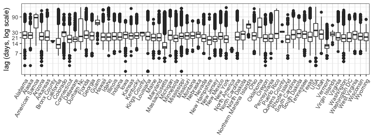
The following figure shows the reporting lags by state as computed in
the data as the difference between the date the sample was taken and
the date_submitted, which is the date the sample was submitted to the
GenBank system. There appears to be substantial variation by location
(note the shorter lags in MA, CA and VT), with 75% of samples typically
reported by 1 month out. Note this is subsetting to look at all data
starting in August of 2021. Some analyses, for example the
Rt analysis that the Bedford Lab has
done, remove all
samples from the last 10 days, to try to remove small sample effects in
the early reporting.
us_dat %>%
  filter(date > ymd("2021-08-01")) %>%
  ggplot(aes(x=division, y=reporting_lag)) +
  geom_boxplot() +
  scale_y_log10(name= "lag (days, log scale)", breaks=c(7, 14, 21, 30, 90, 360, 720)) +
  xlab(NULL) +
  theme(axis.text.x = element_text(angle=60, vjust=1, hjust=1))

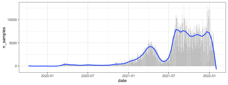
Plot of samples over time
us_dat %>%
  group_by(date) %>%
  summarize(n_samples = n()) %>%
  ggplot(aes(x=date, y=n_samples)) +
  geom_bar(alpha=.3, stat="identity") +
  geom_smooth(span=.1, se=FALSE)

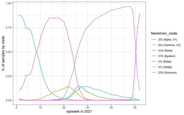
Here is a plot of the prevalence of each clade by week across 2021.
strains_of_interest <-
  c("20I (Alpha, V1)",
    "20J (Gamma, V3)",
    "21A (Delta)",
    "21C (Epsilon)",
    "21I (Delta)",
    "21J (Delta)",
    "21K (Omicron)"
    )

by_clade <- us_dat %>%
  filter(year(date) == 2021) %>%   ## focus only on 2021
  filter(Nextstrain_clade %in% strains_of_interest) %>%
  mutate(epiweek = epiweek(date)) %>%
  filter(epiweek < 53) %>%        ## values of 53 are at the start of 2021
  group_by(Nextstrain_clade, epiweek) %>%
  summarize(clade_total = n()) %>%
  group_by(epiweek) %>%
  mutate(total_samples = sum(clade_total),
         pct_clade_in_epiweek = clade_total/total_samples)

by_clade %>%
  ggplot(aes(x=epiweek, y=pct_clade_in_epiweek, color=Nextstrain_clade)) +
  geom_line() +
  xlab("epiweek in 2021") +
  ylab("% of samples by clade")

We wish to thank all the labs whose effort and time are essential to making these important data available. Also, thanks to Trevor Bedford and the Nextstrain team for providing the processed version of the metadata files and providing some pointers and insights about these data as we were writing this post.